One of the standard applications of orthogonal projections to function spaces comes in the form of Fourier series, where we use \(B = \{1,\cos(x),\sin(x),\cos(2x),\sin(2x),\ldots\}\) as a mutually orthogonal set of functions with respect to the usual inner product

\(\displaystyle\langle f, g \rangle = \int_{-\pi}^\pi f(x)g(x) \, \mathrm{d}x.\)

In particular, projecting a function onto the span of the first 2n+1 functions in the set \(B\) gives its order-n Fourier approximation:

\(\displaystyle f(x) \approx a_0 + \sum_{k=1}^n a_k \cos(kx) + \sum_{k=1}^n b_k \sin(kx),\)

where the coefficients \(a_0,a_1,a_2,\ldots,a_n\) and \(b_1,b_2,\ldots,b_n\) can be computed via inner products (i.e., integrals) in this space (see many other places on the web, like here and here, for more details).

A natural follow-up question is then whether or not we similarly get Taylor polynomials when we project a function down onto the span of the set of functions \(C = \{1,x,x^2,x^3,\ldots,x^n\}\). More specifically, if we define \(\mathcal{C}[-1,1]\) to be the inner product space consisting of continuous functions on the interval [-1,1] with the standard inner product

\(\displaystyle\langle f, g \rangle = \int_{-1}^1 f(x)g(x) \, \mathrm{d}x,\)

and consider the orthogonal projection \(P : \mathcal{C}[-1,1] \rightarrow \mathcal{C}[-1,1]\) with range equal to \(\mathcal{P}_n[-1,1]\), the subspace of degree-n polynomials, is it the case that \(P(e^x)\) is the degree-n Taylor polynomial of \(e^x\)?

It does not take long to work through an example to see that, no, we do not get Taylor polynomials when we do this. For example, if we choose n = 2 then projecting the function \(e^x\) onto the  \(\mathcal{P}_2[-1,1]\) results in the function \(P(e^x) \approx 0.5367x^2 + 1.1036x + 0.9963\), which is not its degree-2 Taylor polynomial \(p_2(x) = 0.5x^2 + x + 1\). These various functions are plotted below (\(e^x\) is displayed in orange, and the two different approximating polynomials are displayed in blue):

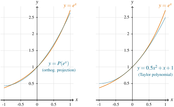
These plots illustrate why the orthogonal projection of \(e^x\) does not equal its Taylor polynomial: the orthogonal projection is designed to approximate \(e^x\) as well as possible on the whole interval [-1,1], whereas the Taylor polynomial is designed to approximate it as well as possible at x = 0 (while sacrificing precision near the endpoints of the interval, if necessary).

However, something interesting happens if we change the interval that the orthogonal projection acts on. In particular, if we let \(0 < c \in \mathbb{R}\) be a scalar and instead consider the orthogonal projection \(P_c : \mathcal{C}[-c,c] \rightarrow \mathcal{C}[-c,c]\) with range equal to \(\mathcal{P}_2[-c,c]\), then a straightforward (but hideous) calculation shows that the best degree-2 polynomial approximation of \(e^x\) on the interval [-c,c] is

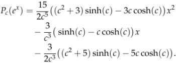
While this by itself is an ugly mess, something interesting happens if we take the limit as c approaches 0:

\(\displaystyle\lim_{c\rightarrow 0^+} P_c(e^x) = \frac{1}{2}x^2 + x + 1,\)

which is exactly the Taylor polynomial of \(e^x\). Intuitively, this makes sense and meshes with our earlier observations about Taylor polynomials approximating \(e^x\) at x = 0 as well as possible and orthogonal projections \(P_c(e^x)\) approximating \(e^x\) as well as possible on the interval \([-c,c]\). However, I am not aware of any proof that this happens in general (i.e., no matter what the degree of the polynomial is and no matter what (sufficiently nice) function is used in place of \(e^x\)), and I would love for a kind-hearted commenter to point me to a reference. [Update: user “jam11249” provided a sketch proof of this fact on reddit here.]

Here is an interactive Desmos plot that you can play around with to see the orthogonal projection approach the Taylor polynomial as \(c \rightarrow 0\).