Archive

Posts Tagged ‘Coding’

How to compute hard-to-compute matrix norms

January 11th, 2016

There are a wide variety of different norms of matrices and operators that are useful in many different contexts. Some matrix norms, such as the Schatten norms and Ky Fan norms, are easy to compute thanks to the singular value decomposition. However, the computation of many other norms, such as the induced p-norms (when p ≠ 1, 2, ∞), is NP-hard. In this post, we will look at a general method for getting quite good estimates of almost any matrix norm.

The basic idea is that every norm can be written as a maximization of a convex function over a convex set (in particular, every norm can be written as a maximization over the unit ball of the dual norm). However, this maximization is often difficult to deal with or solve analytically, so instead it can help to write the norm as a maximization over two or more simpler sets, each of which can be solved individually. To illustrate how this works, let’s start with the induced matrix norms.

Induced matrix norms

The induced p → q norm of a matrix B is defined as follows:

\(\displaystyle\|B\|_{p\rightarrow q}:=\max\big\{\|B\mathbf{x}\|_q : \|\mathbf{x}\|_p = 1\big\},\)

where

\(\displaystyle\|\mathbf{x}\|_p := \left(\sum_{i}|x_i|^p\right)^{1/p}\)

is the vector p-norm. There are three special cases of these norms that are easy to compute:

  1. When p = q = 2, this is the usual operator norm of B (i.e., its largest singular value).
  2. When p = q = 1, this is the maximum absolute column sum: \(\|B\|_{1\rightarrow 1} = \max_j\sum_i|b_{ij}|\).
  3. When p = q = ∞, this is the maximum absolute row sum: \(\|B\|_{\infty\rightarrow \infty} = \max_i\sum_j|b_{ij}|\).

However, outside of these three special cases (and some other special cases, such as when B only has real entries that are non-negative [1]), this norm is much messier. In general, its computation is NP-hard [2], so how can we get a good idea of its value? Well, we rewrite the norm as the following double maximization:

\(\displaystyle\|B\|_{p\rightarrow q}=\max\big\{|\mathbf{y}^*B\mathbf{x}| : \|\mathbf{x}\|_p = 1, \|\mathbf{y}\|_{q^\prime} = 1\big\},\)

where \(q^\prime\) is the positive real number such that \(1/q + 1/q^\prime = 1\) (and we take \(q^\prime = 1\) if \(q = \infty\), and vice-versa). The idea is then to maximize over \(\mathbf{x}\) and \(\mathbf{y}\) one at a time, alternately.

  1. Start by setting \(j = 1\) and fixing a randomly-chosen vector \(\mathbf{x}_0\), scaled so that \(\|\mathbf{x}_0\|_{p} = 1\).
  2. Compute

    \(\max\big\{|\mathbf{y}^*B\mathbf{x}_{j-1}| : \|\mathbf{y}\|_{q^\prime} = 1\big\},\)

    keeping \(\mathbf{x}_{j-1}\) fixed, and let \(\mathbf{y}_j\) be the vector attaining this maximum. By Hölder’s inequality, we know that this maximum value is exactly equal to \(\|B\mathbf{x}_{j-1}\|_{q}\). Furthermore, the equality condition of Hölder’s inequality tells us that the vector \(\mathbf{y}_j\) attaining this maximum is the one with complex phases that are the same as those of \(B\mathbf{x}_{j-1}\), and whose magnitudes are such that \(|\mathbf{y}_j|^{q^\prime}\) is a multiple of \(|B\mathbf{x}_{j-1}|^q\) (here the notation \(|\cdot|^q\) means we take the absolute value and the q-th power of every entry of the vector).

  3. Compute

    \(\max\big\{|\mathbf{y}_j^*B\mathbf{x}| : \|\mathbf{x}\|_{p} = 1\big\},\)

    keeping \(\mathbf{y}_j\) fixed, and let \(\mathbf{x}_j\) be the vector attaining this maximum. By an argument almost identical to that of step 2, this maximum is equal to \(\|B^*\mathbf{y}_j\|_{p^\prime}\), where \(p^\prime\) is the positive real number such that \(1/p + 1/p^\prime = 1\). Furthermore, the vector \(\mathbf{x}_j\) attaining this maximum is the one with complex phases that are the same as those of \(B^*\mathbf{y}_j\), and whose magnitudes are such that \(|\mathbf{x}_j|^p\) is a multiple of \(|B^*\mathbf{y}_j|^{p^\prime}\).

  4. Increment \(j\) by 1 and return to step 2. Repeat until negligible gains are made after each iteration.

This algorithm is extremely quick to run, since Hölder’s inequality tells us exactly how to solve each of the two maximizations separately, so we’re left only performing simple vector calculations at each step. The downside of this algorithm is that, even though it will always converge to some local maximum, it might converge to a value that is smaller than the true induced p → q norm. However, in practice this algorithm is fast enough that it can be run several thousand times with different (randomly-chosen) starting vectors \(\mathbf{x}_0\) to get an extremely good idea of the value of \(\|B\|_{p\rightarrow q}\).

It is worth noting that this algorithm is essentially the same as the one presented in [3], and reduces to the power method for finding the largest singular value when p = q = 2. This algorithm has been implemented in the QETLAB package for MATLAB as the InducedMatrixNorm function.

Induced Schatten superoperator norms

There is a natural family of induced norms on superoperators (i.e., linear maps \(\Phi : M_n \rightarrow M_n\)) as well. First, for a matrix \(X \in M_n\), we define its Schatten p-norm to be the p-norm of its vector of singular values:

\(\|X\|_p := \left(\sum_{i=1}^n \sigma_i(X)^p\right)^{1/p}.\)

Three special cases of the Schatten p-norms include:

  • p = 1, which is often called the “trace norm” or “nuclear norm”,
  • p = 2, which is often called the “Frobenius norm” or “Hilbert–Schmidt norm”, and
  • p = ∞, which is the usual operator norm.

The Schatten norms themselves are easy to compute (since singular values are easy to compute), but their induced counter-parts are not.

Given a superoperator \(\Phi : M_n \rightarrow M_n\), its induced Schatten p → q norm is defined as follows:

\(\|\Phi\|_{p\rightarrow q} := \max\big\{ \|\Phi(X)\|_q : \|X\|_p = 1 \big\}.\)

These induced Schatten norms were studied in some depth in [4], and crop up fairly frequently in quantum information theory (especially when p = q = 1) and operator theory (especially when p = q = ∞). The fact that they are NP-hard to compute in general is not surprising, since they reduce to the induced matrix norms (discussed earlier) in the case when \(\Phi\) only acts on the diagonal entries of \(X\) and just zeros out the off-diagonal entries. However, it seems likely that this norm’s computation is also difficult even in the special cases p = q = 1 and p = q = ∞ (however, it is straightforward to compute when p = q = 2).

Nevertheless, we can obtain good estimates of this norm’s value numerically using essentially the same method as discussed in the previous section. We start by rewriting the norm as a double maximization, where each maximization individually is easy to deal with:

\(\|\Phi\|_{p\rightarrow q} = \max\big\{ |\mathrm{Tr}(Y^*\Phi(X))| : \|X\|_p = 1, \|Y\|_{q^\prime} = 1\big\},\)

where \(q^\prime\) is again the positive real number (or infinity) satisfying \(1/q + 1/q^\prime = 1\). We now maximize over \(X\) and \(Y\), one at a time, alternately, just as before:

  1. Start by setting \(j = 1\) and fixing a randomly-chosen matrix \(X_0\), scaled so that \(\|X_0\|_p = 1\).
  2. Compute

    \(\max\big\{|\mathrm{Tr}(Y^*\Phi(X_{j-1})| : \|Y\|_{q^\prime} = 1\big\},\)

    keeping \(X_{j-1}\) fixed, and let \(Y_j\) be the matrix attaining this maximum. By the Hölder inequality for Schatten norms, we know that this maximum value is exactly equal to \(\|\Phi(X_{j-1})\|_{q}\). Furthermore, the matrix \(Y_j\) attaining this maximum is the one with the same left and right singular vectors as \(\Phi(X_{j-1})\), and whose singular values are such that there is a constant \(c\) so that \(\sigma_i(Y_j)^{q^\prime} = c\sigma_i(\Phi(X_{j-1}))^q\) for all \(i\) (i.e., the vector of singular values of \(Y_j\), raised to the \(q^\prime\) power, is a multiple of the vector of singular values of \(\Phi(X_{j-1})\), raised to the \(q\) power).

  3. Compute

    \(\max\big\{|\mathrm{Tr}(Y_j^*\Phi(X)| : \|X\|_{p} = 1\big\},\)

    keeping \(Y_j\) fixed, and let \(X_j\) be the matrix attaining this maximum. By essentially the same argument as in step 2, we know that this maximum value is exactly equal to \(\|\Phi^*(Y_j)\|_{p^\prime}\), where \(\Phi^*\) is the map that is dual to \(\Phi\) in the Hilbert–Schmidt inner product. Furthermore, the matrix \(X_j\) attaining this maximum is the one with the same left and right singular vectors as \(\Phi^*(Y_j)\), and whose singular values are such that there is a constant \(c\) so that \(\sigma_i(X_j)^{p} = c\sigma_i(\Phi^*(Y_j))^{p^\prime}\) for all \(i\).

  4. Increment \(j\) by 1 and return to step 2. Repeat until negligible gains are made after each iteration.

The above algorithm is almost identical to the algorithm presented for induced matrix norms, but with absolute values and complex phases of the vectors \(\mathbf{x}\) and \(\mathbf{y}\) replaced by the singular values and singular vectors of the matrices \(X\) and \(Y\), respectively. The entire algorithm is still extremely quick to run, since each step just involves computing one singular value decomposition.

The downside of this algorithm, as with the induced matrix norm algorithm, is that we have no guarantee that this method will actually converge to the induced Schatten p → q norm; only that it will converge to some lower bound of it. However, the algorithm works pretty well in practice, and is fast enough that we can simply run it a few thousand times to get a very good idea of what the norm actually is. If you’re interested in making use of this algorithm, it has been implemented in QETLAB as the InducedSchattenNorm function.

Entanglement Norms

The central idea used for the previous two families of norms can also be used to get lower bounds on the following norm on \(M_m \otimes M_n\) that comes up from time to time when dealing with quantum entanglement:

\(\|X\|_{S(1)} := \max\Big\{\big|(\mathbf{v}\otimes\mathbf{w})^*X(\mathbf{x} \otimes \mathbf{y})\big| : \|\mathbf{v}\| = \|\mathbf{w}\| = \|\mathbf{x}\| = \|\mathbf{y}\| = 1\Big\}.\)

(As a side note: this norm, and some other ones like it, were the central focus on my thesis.) This norm is already written for us as a double maximization, so the idea presented in the previous two sections is somewhat clearer from the start: we fix randomly-generated vectors \(\mathbf{v}\) and \(\mathbf{x}\) and then maximize over all vectors \(\mathbf{w}\) and \(\mathbf{y}\), which can be done simply by computing the left and right singular vectors associated with the maximum singular value of the operator

\((\mathbf{v} \otimes I)^*X(\mathbf{x} \otimes I) \in M_n.\)

We then fix \(\mathbf{w}\) and \(\mathbf{y}\) as those singular vectors and then maximize over all vectors \(\mathbf{v}\) and \(\mathbf{x}\) (which is again a singular value problem), and we iterate back and forth until we converge to some value.

As with the previously-discussed norms, this algorithm always converges, and it converges to a lower bound of \(\|X\|_{S(1)}\), but perhaps not its exact value. If you want to take this algorithm out for a spin, it has been implemented in QETLAB as the sk_iterate function.

It’s also worth mentioning that this algorithm generalizes straightforwardly in several different directions. For example, it can be used to find lower bounds on the norms \(\|\cdot\|_{S(k)}\) where we maximize on the left and right by pure states with Schmidt rank not larger than k rather than separable pure states, and it can be used to find lower bounds on the geometric measure of entanglement [5].

References:

  1. D. Steinberg. Computation of matrix norms with applications to robust optimization. Research thesis. Technion – Israel University of Technology, 2005.
  2. J. M. Hendrickx and A. Olshevsky. Matrix p-norms are NP-hard to approximate if p ≠ 1,2,∞. 2009. E-print: arXiv:0908.1397
  3. D. W. Boyd. The power method for ℓp norms. Linear Algebra and Its Applications, 9:95–101, 1974.
  4. J. Watrous. Notes on super-operator norms induced by Schatten norms. Quantum Information & Computation, 5(1):58–68, 2005. E-print: arXiv:quant-ph/0411077
  5. T.-C. Wei and P. M. Goldbart. Geometric measure of entanglement and applications to bipartite and multipartite quantum states. Physical Review A, 68:042307, 2003. E-print: arXiv:quant-ph/0212030

The Maximal Lifespan of Patterns in Conway's Game of Life

July 31st, 2009

In a couple of recent posts, I argued that random patterns in Conway’s Game of Life tend, on average, to live longest when they have an initial density of 37.5% cells being alive. In this post, rather than looking at the distribution of the average lifespan for various initial densities, I will fix the density at 37.5% and look at the distribution of lifespans that results, and use that to estimate what the maximal lifespan of any small pattern is (as in my previous posts, I will use 20×20 starting patterns). As before, I will explore both the case when we simulate Life on a torus and when we simulate it on an infinite plane.

Lifespan Distribution on a Torus

After simulating 175000 random patterns on a 20×20 torus, the distribution of the lifespans was as follows:

Lifespan Frequency Histogram on a TorusThe bins in the graph have a width of 10, and the peak occurs in the lifespan 91 – 100 bin. Some other interesting stats include:

  • Maximum observed lifespan: 2092
  • Minimum observed lifespan: 14
  • Average lifespan: 210
  • Median lifespan: 164
  • Standard deviation of lifespan: 159.3

In order to try to estimate the longest lifespan of any pattern on a 20×20 torus, I will assume that if the lifespan is above 100, then it follows an exponential distribution, which appears to be a reasonable assumption given the above histogram. Indeed, this leads to the following histogram, which has the exponential of best fit overlaid in black. The equation of the exponential is y = 9088.7(0.938)x, and the R2 value is 0.997 (that’s one heck of a good fit).

Lifespan Frequency Trend on a TorusNow that we have our exponential of best fit, we can get an estimate of the maximal lifespan in this scenario by assuming that the lifespan of the 220*20 different patterns are independent of each other (this may not be a particularly good assumption, as two patterns, for example, will have the same lifespan if they are translations of each other — nonetheless it seems that the number of reductions that can be made by symmetry arguments like that is tiny compared to the total number of such patterns, so let’s roll with it). We then set

Torus equation

and solve for x to get a maximal lifespan of x = 4474. This seems believable and not particularly shocking to me given the statistics that I listed earlier.

Lifespan Distribution on a Plane

Typically, Life enthusiasts are more interested in results on the infinite plane than on a torus, as it leads to behaviour that is much more chaotic and unpredictable. For example, even though we just saw that the longest-lived 20×20 pattern on a torus likely lives for less than 4500 generations, there is a known 9×15 pattern that lives on the plane for over 29000 generations. We will now proceed analogously to the torus discussion above to see how much better we can reasonably expect to do. We begin with the distribution of the lifespan based on 60000 initial 20×20 patterns:

Lifespan Frequency Histogram on a Plane

The bins in the graph have a width of 50, and the peak occurs in the lifespan 151 – 200 bin. The other basic stats are listed below, and as we would expect, the average lifespan and the standard deviation of lifespans are both much greater on the plane than they are on the torus.

  • Maximum observed lifespan: 13612
  • Minimum observed lifespan: 15
  • Average lifespan: 678
  • Median lifespan: 368
  • Standard deviation of lifespan: 885.6

The main difference with the analysis in this situation is that instead of assuming the lifespan itself follows an exponential distribution, I will assume that some power of the lifespan follows an exponential distribution; the reason for this is that the R2 is quite low if we try to fit an exponential to the distribution of the lifespans itself. Fitting an exponential to lifespan0.75 seems to give the maximum R2 value (0.9857), so this is what I will use. The following histogram shows the curve of best fit, which has the equation y = 1854.6(0.957)x, where this time x = lifespan0.75.

Lifespan Frequency Trend on a Plane

Finally, we follow our method from before and set

Lifespan on a Plane Equation

and solve for x to get a maximal lifespan of x = 120795. Of course, this number should be taken with a grain of salt, because that pattern I mentioned earlier that has a lifespan of over 29000 generations was found during a simulation of a whopping 12 billion 20×20 patterns, while our equation of best fit tells us that after 12 billion patterns, we would expect only to see a pattern with lifespan 6206 (when really it should only take about 400 patterns to see such a lifespan). Similarly, in the longest-lived patterns found by the Online Life-Like CA Soup Search, a pattern has been found with lifespan 24389. According to our formula, we should have to look at roughly 9 million billion billion billion soups before finding such a pattern, but only 40 million soups have actually been searched.

This all seems to suggest that the longest-lived pattern in a 20×20 box may in fact live considerably longer than 120000 generations, which goes to show just how in the dark we are when it comes to some of these simple questions — since the search space is so unimaginably huge, we likely will never know for sure what the true upper limit is.

Downloads:

Longevity in Conway's Game of Life Revisited

July 17th, 2009

A couple of weeks ago, I posted some intuition that suggested that, in Conway’s Game of Life, the longest-lived patterns should on average be those with density right around 37.5%. To test this hypothesis, I wrote a simple Golly Python script that generated random 20×20 patterns of varying densities and checked how long it took for them to stabilize. One noticeable problem cropped up, however: patterns with density around 90% tended to live for an extremely long time due to edge effects that caused the pattern to explode out of the original 20×20 box initially, even though they would almost entirely die off within the box.

The solution to the given problem is to emulate the Game of Life not on an infinite planar grid, but rather on a toroidal grid; that is, we fix our 20×20 universe and treat the top row as if it borders the bottom row and the left row as if it borders the right row. Running the simulation in this set-up results in data that matches our intuition more closely:

Lifespan on a TorusThe results are based on 13592 random patterns of each density 1%, 2%, 3%, …, 99%. As with the previous graph, we notice that the lifespan plateaus in the 25% – 50% range, providing evidence that our intuition for a maximum at 37.5% is probably well-founded. Also, at the request of Elithrion in the comments on the previous post, I have included the median plot for the lifespans this time as well, though the median seems to behave pretty similarly to the average (it’s just more or less uniformly 25% smaller). As we would expect, the average lifespan in the toroidal universe set-up is much lower than the average lifespan in the infinite planar grid set-up, because expanding patterns have nowhere to go. The longest-lived pattern that was found on the torus had a lifespan of 2169 (and an initial density of 30%), whereas the longest-lived pattern that was found on the infinite plane (over significantly fewer trials, I might add) was 14042.

While I’m presenting results, how about we take a look at the final population of patterns of various starting densities?

Torus final populationThe behaviour is almost identical to that of the average/median lifespan. The one cool thing is that, in addition to the plateau centred at ~37.5%, here we see that the median final population peaks with a value of 13 at an initial density of 38%. Nevermind the fact that this is almost certainly a statistical anomaly — it helps support my original hypothesis, and if the popular news media has taught me anything, it’s that randomly picking out things like that and claiming that they are significant is always mathematically sound.

Downloads:

The Online Life-Like CA Soup Search

July 11th, 2009

UPDATE [April 17, 2015]: The Online Life-Like CA Soup Search has been offline for some time now (due to being written in ASP, and me now only running websites on Linux hosts, which means I would have to re-code it entirely in PHP). However, I am happy to announce that Adam P. Goucher has recently released a new distributed soup search script called Catagolue. Not only is this script much faster than mine, but it also has many other improvements, such as being (much) better at distinguishing different objects that are near each other, and being more cryptographically secure.

See this forum thread for the announcement as well as some discussion of discoveries made by the search so far.


Today I’m “officially” announcing the Online Life-Like CA Soup Search, though some of the folks over at the ConwayLife.com forums have been helping me test it out for a couple of weeks now.

As I mentioned in this post, one way to learn about the general behaviour of Conway’s Game of Life (or any other Life-like cellular automaton) is to generate random patterns and see what stable patterns they typically evolve into (if any). If you’ve played around with Conway’s Game of Life, then you more than likely are very familiar with blocks, blinkers, beehives, loaves, and maybe even pulsars, simply as a result of drawing random gibberish on the grid and letting it evolve. This is exactly the idea behind the Online Life-Like CA Soup Search, just on a larger scale — what if we had lots of people’s computers drawing random gibberish on Life grids, letting them evolve, and storing the resulting patterns in a communal database?

This method of collecting patterns in Life is known as a census, and to my knowledge it has been carried out on a relatively large scale twice in the past; once by Achim Flammenkamp (results here), and once by Andrej Okrasinski (results linked in the first paragraph here). As we would expect, the block is by far the most common still life, and the blinker is by far the most common oscillator. If we scroll down a bit, we see that the pulsar is the fourth most common oscillator (which is reasonably surprising, given its size). Scrolling much past that, we get into the interesting stuff — objects that no reasonable person has ever seen from drawing random stuff and seeing what it evolves into, simply because they occur so infrequently.

So why bother doing another census if two rather large-scale censuses (censi?) have already been carried out? My reasons are threefold:

  1. There has never (to my knowledge) been a census of any other Life-like cellular automata conducted. The Online Life-Like CA Soup Search is completely general in that it can conduct a census of any Life-like rule (assuming that rule is stable, of course). Censuses have already been started for five other rules, including 2×2, Day & NightHighLife, and Move. Because some of these other rules have been studied relatively little, this is an easy way of discovering new yet fundamental patterns in them. For example, it didn’t take long for the soup search script to uncover a c/8 line puffer in the 2×2 (B36/S125) rule; the very first known pattern that exhibits infinite growth in 2×2!

    Line puffer in 2x2

    Line puffer in 2×2

  2. Previous soup searches were limited in that they only looked for very specific types of objects — usually still lifes and oscillators (though Achim Flammenkamp did a search for spaceships and puffers that can be viewed here). The Online Life-Like CA Soup Search searches for still lifes, oscillators, spaceships and puffers all at once, and even gets pseudo objects (such as the bi-block) as well.
  3. Multiple users can run the script and contribute to the results simultaneously. Rather than just having one person run a script that they themself wrote, the Online Life-Like CA Soup Search works by having users download a script and that script uploads results to the central database. This obviously provides a huge speed-up, and allows the census to continuously improve and expand.

So what are you waiting for? Visit the Online Life-Like CA Soup Search, download the script, and put your computer’s CPU cycles to good use!

Census results in Conway's Game of Life

Census results in Conway’s Game of Life

Longest-Lived Soup Density in Conway's Game of Life

June 26th, 2009

In Conway’s Game of Life, a simple way to learn about the general dynamics of the game are to study what happens to soup – patterns made up of a random assortment of ON and OFF cells. Two particularly interesting questions that we can ask are “What types of stable patterns arise most frequently from soup?” and “How long does soup generally last before stabilizing?” I will focus on the latter question for today’s post, as the former has become the bud of a more ambitious project that I will announce in the near future.

The question of how long soup generally lasts before stabilizing is quite vague, because there are two important considerations that we have not specified:

  1. How dense should the soup be? Clearly soup with ON density of 5% will survive only a fraction as long as soup with ON density of 50%.
  2. How large of a region of soup should we let evolve? Smaller regions will stabilize much more quickly than large regions, and infinite regions will likely never stabilize(?), not to mention we can’t effectively simulate an infinite field of random cells.

For #2, I will choose the region to be of size 20×20. This decision is pretty arbitrary, but part of the reason I chose such a small size is as a desire to make this script kill two birds with one stone; any particularly long-lived patterns of this size that are discovered can likely be considered methuselahs, while larger patterns can not.

For #1, we might naively expect that patterns will live longest if they have density 37.5%, since cells are born if and only if they have exactly three ON neighbours (out of a possible eight = 37.5%). To test this theory, I created a Golly script that creates regions of varying density and checks how long it takes for them to stabilize. The following graph shows the average lifespan of 20×20 patterns with densities ranging from 1% to 99%, based on 5000 generated patterns for each percentage point.

Average lifespan after 5000 trials

Indeed, it looks like the longest-lived density estimate of 37.5% isn’t too far off. The true maximum in this set-up might actually be slightly higher, but that is most likely caused by the same thing that is causing the hump centered at 90%: edge effects. Roughly speaking, because we are simulating a finite region of soup on an infinite grid (as opposed to on a toroidal universe), patterns of higher density will tend to expand out very quickly in their first few generations, giving them longer lifespans in general than they would have on a toroidal universe. Alas, Golly doesn’t support toroidal universes, so the toroidal lifespan results will have to wait for another day.

Update [July 8, 2009]: I have attached to the end of this post the Python script used to generate these results.

Update [July 11, 2009]: See this post, which deals with the “more ambitious project” that I mentioned.

Update [July 19, 2009]: See this post, which deals with soup longevity on a torus.

Downloads:

On Maximal Self-Avoiding Walks

May 5th, 2009

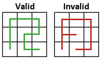
Given a k × n grid, a self-avoiding walk (SAW) on that grid is a connected path that never touches the same square more than once and never doubles back on itself (note that some sources make the convention that the path is drawn on the edges of the grid from vertex to vertex, but here I will make the convention that the path connects the centres of the squares that the grid forms). I will define a maximal self-avoiding walk to be a self-avoiding walk that touches every square of the grid on which it resides. One natural question that we can ask in this setting is “How many maximal self-avoiding walks are there on a k × n grid?”

Before proceeding, let’s simplify things slightly by making the restriction that the maximal self-avoiding walks must start in the bottom-left corner of the grid (this restriction leaves us with the walks that are known as “Greek-key tours”). Let f(k, n) denote the number of maximal self-avoiding walks on a k × n grid. Unfortunately, finding an expression for f(k, n) in complete generality seems to be out of reach, so we will instead try to answer the question for certain fixed values of k.
Case 1: k = 1
Regardless of n, there is clearly only one maximal self-avoiding walk in this case: a straight line. Thus, f(1, n) = 1 regardless of the value of n.

Case 2: k = 2
It is not difficult to prove (by induction, for example) that f(2, n) = n.

Case 3: k = 3
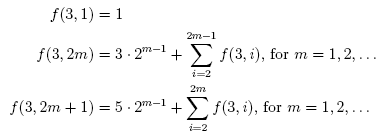
This is the first case whose solution does not seem trivial. It is well-known (by people who have looked at this problem, anyways) that the number of maximal self-avoiding walks on a 3 × n grid for n = 1, 2, … is 1, 3, 8, 17, 38, … (Sloane’s A046994). This sequence is defined by the following recurrence relations:

Well, from these recurrence relations we can derive the following closed form expression for f(3, n):

It may be worth noting that this formula can be simplified significantly if you consider the case when n is odd separately from the case when n is even, and write f(3, n) as a branch function.

Case 4: k = 4
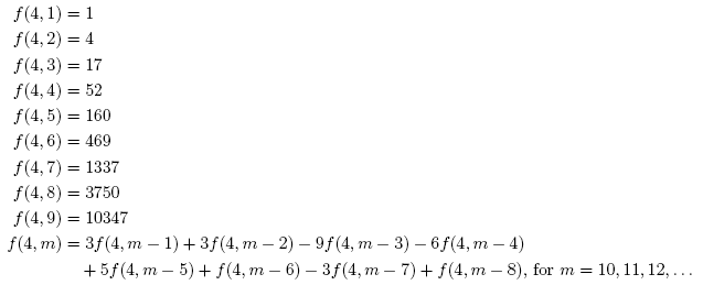
The number of maximal self-avoiding walks on a 4 × n grid for n = 1, 2, … is 1, 4, 17, 52, 160, … (Sloane’s A046995), but to date no simple closed-form formula for f(4, n) has been found. In 2003, Dean Hickerson proposed the following recurrence relation to define f(4, n), which holds at least for the first 25 terms of the sequence:

While it is possible to derive a closed-form formula for f(4, n) from the above recurrence relation using standard difference equation techniques, the formula is extremely long and cumbersome. One piece of information that we can extract from the closed-form formula (which I won’t write out here) is that f(4, n) ∈ O(2.539n).

Case 5: k ≥ 5
It is now clear that this problem grows very large very quickly, and proceeding in this manner may not be (realistically) feasible. Not much is known about f(k, n) when both k and n are greater than or equal to 5. The best approach in this case is likely that of brute force.

Computing the Number of Maximal SAWs

Here I provide two programs for computing the number of maximal SAWs on a grid of your chosen size. It is recommended that you use the C script rather than the Visual Basic program, as the C script is much faster.

If the Visual Basic file below gives you an error message when you try to run it, you may need to download and install the Visual Basic 6.0 run time files. Click here to download these files. As far as I know, this program should work on Windows 98, ME, 2000, XP and Vista, but I can’t make any guarantees about its compatability.

Download:

Maximal SAW Table of Values

This is a table giving the number of maximal SAWs on a k × n grid. Several of the values in the table below were calculated using the above software — the cells that have “?” in them correspond to values that are currently unknown due to computational limits. Note that there is trivially symmetry across the main diagonal of the table. I apologize for the unreadably small font.

k\n 1 2 3 4 5 6 7 8 9 10 General Term
1 1 1 1 1 1 1 1 1 1 1 1
2 1 2 3 4 5 6 7 8 9 10 n
3 1 3 8 17 38 78 164 332 680 1368 Sloane’s A046994
4 1 4 17 52 160 469 1337 3750 10347 28249 Sloane’s A046995
5 1 5 38 160 824 3501 16262 68591 304177 1276805 Sloane’s A145156
6 1 6 78 469 3501 22144 144476 899432 5585508 34092855 Sloane’s A160240
7 1 7 164 1337 16262 144476 1510446 13506023 132712481 1185979605 Sloane’s A160241
8 1 8 332 3750 68591 899432 13506023 180160012 ? ? ?
9 1 9 680 10347 304177 5585508 132712481 ? ? ? ?
10 1 10 1368 28249 1276805 34092855 1185979605 ? ? ? ?
n × n grid: Sloane’s A145157

Update (August 7, 2024): Jay Pantone, Alexander R. Klotz, and Everett Sullivan have written a great paper that (among other things) significantly expands these results.

Related Links: