I presented the labs for the first-year calculus course at my school this past semester, and as a bit of an experiment I decided to try giving the students some less “ordinary” problems to work on at the end of the labs (partly inspired by this problem). I only ended up doing it for the first four weeks of the semester due to a combination of it taking much too long to create them and a general lack of interest by most of the students, but they were fun to make anyway so I might as well share them in case anyone else would like to present these or similar problems in their own labs or course. PDF as well as TeX files are provided, so you can edit out my name and all that jazz.

Lab #1: Intervals with Braid

The first week’s problem was based off the video game Braid. This problem ended up not working too well due to about 10 people in the class of ~600 having played of the game, and the rest being very confused by the idea of the cloud platform moving along with the main character (it makes sense if you’ve played the game, honest!).

Download: Question sheet [pdf], Solution sheet [pdf], TeX files [zip]

Lab #2: The Bat Man

The next week I decided to go a bit more mainstream and have the problem based on Batman chasing the Joker. The question doesn’t make a lick of sense if you think about it physically (the cars have negative acceleration for one thing), but this being a math class I decided not to care. I feel like this was the most successful of the weekly problems because the Batman/Joker stuff was completely incidental and the question was still easy enough for the students to understand and tackle.

Download: Question sheet [pdf], Solution sheet [pdf], TeX files [zip]

Lab #3: Calvin Reaches his Limit

By this point I had learned that even if I am going to sugar-coat the question under a picture of Calvin and Hobbes, it’s a good idea to include a sentence at the end summarizing what the heck it is I’m asking them to compute or prove. I think this is a fun question no matter how advanced of a mathematician you are, and it was probably a bit mean of me to present it to first-year students.

Download: Question sheet [pdf], Solution sheet [pdf], TeX files [zip]

Lab #4: Continuity with Mario

The last of these problems that I presented was a (very) simple continuity question based on Super Mario World. I originally wanted to use Super Metroid for this question since it would allow for more varied movements from the hero, but I decided that (as I learned in Lab #1) it would be best to stick with a more recognizable game. It was a pain to come up with a semi-nice-looking branch function that resembled Mario’s movement in a believable way and led to simple (i.e., non-fractional) limits at the points of interest.

Download: Question sheet [pdf], Solution sheet [pdf], TeX files [zip]

A few months ago, I spent two posts describing the Choi-Jamiolkowski isomorphism between linear operators from M_n to M_m (often referred to as “superoperators“) and linear operators living in the space M_n ⊗ M_m. However, there is another isomorphism between superoperators and regular operators — one that I’m not sure of any name for but which has just as many interesting properties.

Recall from Section 1 of this post that any superoperator Φ can be written as

for some operators {A_i} and {B_i}. The isomorphism that I am going to focus on in this post is the one given by associating Φ with the operator

The main reason that M_Φ can be so useful is that it retains the operator structure of Φ. In particular, if you define vec(X) to be the vectorization of the operator X, then

In other words, if you treat X as a vector, then M_Φ is the operator describing the action of Φ on X. From this it becomes simple to compute some basic quantities describing Φ. For example, the induced Frobenius norm,

is equal to the standard operator norm of M_Φ. If n = m then we can define the eigenvalues {λ} and the eigenmatrices {V} of Φ in the obvious way via

Then the eigenvalues of Φ are exactly the eigenvalues of M_Φ, and the corresponding eigenvectors of M_Φ are the vectorizations of the eigenmatrices of Φ. It is similarly easy to check whether Φ is invertible (by checking whether or not det(M_Φ) = 0), find the inverse if it exists, or find the nullspace (and a pseudoinverse) if it doesn’t.

Finally, here’s a question for the interested reader to think about: why is the transpose required on the B_i operators for this isomorphism to make sense? That is, why can we not define an isomorphism between Φ and the operator

The term “infographic” is a ridiculous little buzzword that really took off on the internet sometime last year. It used to refer to genuinely useful things like subway maps and blueprints. Recently, however, the term has come to mean “an obnoxiously oversized image that has numbers on it”. My problem isn’t with infographics like these ones that just display some fun, meaningless information is a visual way, or this one that displays a phenomenon that is inherently visual. My beef is with infographics that reduce a variety of related statistics to an oversized mess of overlapping graphs and charts that are (purposely or otherwise) misleading.

This post will present four rules that infographic designers, if they decide that they absolutely must make an infographic, should always follow (but often don’t). To get the ball rolling, let’s consider an example that made its way around the internet just a couple of weeks ago (source):

American 2009 Season Premieres and Averages to Date (click to enlarge)

We are told that the above infographic depicts the US viewership for a variety of shows during their premiere (light red) and on average since they began their 2009 season (dark red). However, I have two main problems with the image, and they’re both problems that are prevalent throughout many infographics and can easily be solved by just using a simple bar graph.

1. Infographics should not require horizontal scrolling. The above infographic is 3133 pixels wide, which means there is no consumer-available monitor in the world capable of displaying the entire image on one screen without scrunching it down. This is apparently exactly what infographic makers want, since they all seem to subscribe to the school of thought that dictates their image deserves 45 inches of horizontal viewing space. This would be fine if infographics were readable when zoomed out, but by their very nature they almost never are.

Computer monitors were not meant to view posters. If you want to make the image high-resolution enough that it can be printed out as a poster then it should be created as a vector graphic, not a raster graphic. If you still insist that your infographic should be a monstrously large bitmap, make it readable from a zoom level that will fit on standard monitor resolutions.

Some other popular infographics that suffer from this problem are the new auto industry breakdown, weight of the world, and the first 100 days.

2. Two-dimensional figures should never be used to compare linear data. The above infographic compares the number of people watching different shows, so why are circles being used to represent the data? What represents the number of viewers — the radius of the circle or the area of the circle? The source doesn’t tell us, so we have no way of appropriately assessing how many more people are viewing NCIS: Los Angeles than The Good Wife. If it’s the radius of the circle, NCIS appears to have about 5% more viewers. If it’s the area of the circle then it’s probably over 10% (and the discrepancy gets much larger if you compare shows that are farther apart).

Furthermore, even if we were told whether it’s the radii of the circles or their areas that we should be looking at, there’s still a problem. If the radii are what are being compared, then the visual is misleading because the differences in areas cause the relative differences to appear larger than they actually are. If the areas are what are being compared, then it should be noted that people just plain suck at visually comparing areas. By looking at the above image (and not getting out a ruler or anything) can you tell which circles have about half as much area as the NCIS: Los Angeles circle? Can you tell how much higher the viewership of The Good Wife is than that of Glee? I certainly can’t, at least not quickly.

InfomationIsBeautiful.net is a particularly notorious violator of this rule, as these three examples show: deadliest drugs, how safe is the HPV vaccine?, reduce your chances of dying in a plane crash (scroll down to the “bad month” and “the odds” sections). What’s worse is they aren’t even consistent with whether it’s the areas of the circles or the radii of the circles they’re comparing.

Problems #1 and #2 can both be rectified by simply turning the data into a bar graph. A plain old-fashioned bar graph. Voila:

American 2009 Season Premieres and Averages to Date (easier to read)

The above bar graph doesn’t need to be zoomed in to be read, it makes it easier to compare the relative viewership of each show, and it actually contains more data than the previous infographic thanks to the labels on the vertical axis.

The next example (source) supposedly explains how and why low-cost airlines are able to offer flights that are so much cheaper than other airlines. It made its rounds this last spring during recession fever, when anything that had anything to do with something being cheap was instantly popular. While it does not suffer from problem #1 above (since it is readable when zoomed out), it suffers from two instances of problem #2 as well as multiple other problems.

How come cheap airlines are so cheap? (click to enlarge)

3. Infographics (and everything else) should be about substance over style. While there’s no denying that the above infographic is pretty, does it actually tell us anything? Beyond the myriad of small problems such as the average fare of Southwest flights including cents when none of the other numbers do, the misspelling of “Aer Lingus” and “maintenance”, and the mysterious 43% “total advantage” at the bottom that seems to pop out of nowhere, the infographic at its core doesn’t even make sense.

As the infographic itself says, low-cost airlines generally don’t do long-haul flights; they focus on short point-to-point routes. So why are their average fares being compared to the average fares of the likes of British Airways, who regularly do intercontinental flights? Doesn’t it make sense that travel distance makes more of a contribution to the price of the flight than whether or not tickets are sold primarily online? Average fare per kilometer travelled would make more sense to compare, though it would still be misleading because take-off and landing are disproportionately expensive.

Another recent offending infographic that just simply doesn’t say a thing is the $400 million club, which notes that Transformers: Revenge of the Fallen is only the ninth movie in history to gross more than $400 million at the box office in the US during its theatrical run. The infographic then compares the other eight movies, which of course are juggernauts like Star Wars and Titanic. The problem is that none of the figures are adjusted for inflation. If you scale the numbers properly, Transformers: Revenge of the Fallen actually comes in as about the 65th highest-grossing movie. Impressive, sure, but to say that the infographic is misleading is an understatement.

I will finish by presenting a graphic that ran on NewsWeek.com that shows obesity and “life evaluation” trends over the last year or two. It’s debatable whether or not it falls into the category of what most people would consider an “infographic”, but it perfectly illustrates a core problem with them.

4. Be careful with your data. Just making your graphic pretty doesn’t give you free reign to ignore basic statistical principles when presenting data. In the above graphic, the left graph shows two lines — one showing how many people have BMI less than or equal to 30 in a given month and one showing how many people have BMI over 30 in a given month. I have a news flash for you, NewsWeek: one of those lines is redundant. Not only that, but the redundant second line manipulates the reader by giving the false impression that the number of obese people is converging toward the number of non-obese people. Nevermind the fact that the vertical scale is completely out of whack and it jumps a vertical distance of 46.4% in the same amount of space that is used to represent about a 2.5% jump elsewhere.

I’m willing to bet that the vertical scale on the right graph is completely out of whack too, but it’s a little difficult to tell since they don’t tell you what percentages any of the intermediate y-values correspond to. On the blue “struggling” line, we are given a value of 48.4% on the left edge of the graph and a value of 49.6% at the right edge of the graph at a nearly identical height. Are we supposed to be able to tell how high and low the peaks in the middle of the graph are based on that? Does the blue line get as low as 40%? 35%? 30%? Would labels along the vertical axis (similar to the bar graph I showed above) really have detracted from the desired aesthetic too much?

So if you have a set of data that you wish to convey graphically, please first consider whether or not it can be presented by a simple bar graph or line graph. If it can, don’t try to make it more complicated than that. If it can’t, at least make sure that the information is the motivating factor in your decisions. If the layout ends up dictating how you present your data, you’ve got your priorities backward.

Recently, a family of vector norms [1,2] have been introduced in quantum information theory that are useful for helping classify entanglement of quantum states. In particular, the Schmidt vector k-norm of a vector v ∈ Cⁿ ⊗ Cⁿ, for an integer 1 ≤ k ≤ n, is defined by

In the above definition, SR(w) refers to the Schmidt rank of the vector w and so these norms are in some ways like a measure of entanglement for pure state vectors. One of the results of [2] shows how to compute these norms efficiently, so with that in mind we can perform all sorts of fun numerical analysis on them. Analytic results are provided in the paper, so I’ll provide more hand-wavey stuff and pictures here. In particular, let’s look at what the distributions of the Schmidt vector norms look like.

Figure 1: The distribution of the Schmidt 1 and 2 vector norms in (3 ⊗ 3)-dimensional space

Figure 1 shows the distributions of the Schmidt 1 and 2 norms of unit vectors distributed according to the Haar measure in C³ ⊗ C³, based on 5×10⁵ vectors generated randomly via MATLAB. Note that the Schmidt 3-norm just equals the standard Euclidean norm so it always equals 1 and is thus not shown. Figures 2 and 3 show similar distributions in C⁴ ⊗ C⁴ and C⁵ ⊗ C⁵.

Figure 2: The distribution of the Schmidt 1, 2, and 3 vector norms in (4 ⊗ 4)-dimensional space

Figure 3: The distribution of the Schmidt 1, 2, 3, and 4 vector norms in (5 ⊗ 5)-dimensional space

The following table shows various basic statistics about the above distributions. I suppose the natural next step is to ask whether or not we can analytically determine the distribution of the Schmidt vector norms. Since these norms are essentially just the singular values of an operator that is associated with the vector, it seems like this might even already be a (partially) solved problem, since many results are known about the distribution of the singular values of random matrices. The difficulty comes in trying to interpret the Haar measure (or any other natural measure on pure states, such as the Hilbert-Schmidt measure) on the associated operators.

References:

1. D. Chruscinski, A. Kossakowski, G. Sarbicki, Spectral conditions for entanglement witnesses vs. bound entanglement, Phys. Rev A 80, 042314 (2009). arXiv:0908.1846v2 [quant-ph]
2. N. Johnston and D. W. Kribs, A Family of Norms With Applications in Quantum Information Theory. Journal of Mathematical Physics 51, 082202 (2010). arXiv:0909.3907 [quant-ph]

Those of you familiar with Conway’s Game of Life probably know of its two most basic spaceships: the glider and the lightweight spaceship (shown below). The glider travels diagonally by one cell every four generations (and thus its speed is said to be “c/4”) and the lightweight spaceship travels orthogonally by two cells every four generations (and so its speed is denoted by “2c/4” or “c/2”).

The glider

Lightweight spaceship

A natural question to ask is whether or not there are any spaceships that travel faster than c/4 diagonally or c/2 orthogonally. John Conway proved in 1970 (very shortly after inventing the Game of Life) that the answer is no. I present this proof here, since it’s a bit difficult to find online (though Dave Greene was kind enough to post a copy of it on the ConwayLife.com forums).

Theorem 1. The maximum speed that a spaceship can travel in Conway’s Game of Life is c/4 diagonally and c/2 orthogonally.

Proof. We begin by proving the c/4 speed limit for diagonal spaceships. Consider the grid given in Figure 1 (below). If the spaceship is on and to the left of the diagonal line of cells defined by A, B, C, D, and E in generation 0, then suppose that cell X can be alive in generation 2.

Figure 1: The spaceship is to the left of A, B, C, D, and E

Well, if cell X is alive in generation 2, then cells C, U, and V must be alive in generation 1. This means that U and V must have had 3 alive neighbours in generation 0, so each of B, C, D, J, and K must be alive in generation 0. This means that C must have at least four live neighbours in generation 0 though, so there is no way for it to survive to generation 1, which gives a contradiction.

It follows that X can not be alive in generation 2. In other words, if the spaceship is behind the diagonal line A, B, C, D, E in generation 0, then it must be behind the diagonal line defined by U and V in generation 2. It follows that can not travel faster than c/4 diagonally.

To see the corresponding result for orthogonal spaceships, just use two diagonal lines as in Figure 2. If a spaceship is on and below the diagonal lines defined by the solid black cells in generation 0, then we already saw that it must be on and below the diagonal lines defined by the striped cells in generation 2. It follows that it can not travel faster than c/2 orthogonally.

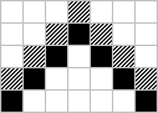
Figure 2: The spaceship is on and below the solid black cells in generation 0

Notice that this result doesn’t only apply to spaceships, but also to other configurations that are (initially) finite and travel across the grid, such as puffers and wickstretchers. Also, this result applies to many Life-like cellular automata — not just Conway’s Game of Life.

In particular, these speed limits apply to any of the 2¹² = 4096 Life-like cellular automata in the range B3/S – B345678/S0123678. That is, these speed limits apply to any rule on the 2D square lattice such that birth occurs for 3 neighbours but not 0, 1, or 2 neighbours, and survival does not occur for 4 or 5 neighbours. But are the spaceship speed limits attained in each of these rules? The regular c/4 glider only works in the 2⁸ = 256 rules from B3/S23 – B3678/S0235678. In the remaining rules, not much is known; some of them have c/3 orthogonal spaceships, some have c/5 orthogonal spaceships, and some have no spaceships at all (such as any of the rules containing S0123, which can not contain spaceships because the trailing edge of the spaceship could never die). Of particular interest are the sidewinder and this spaceship, which play the c/4 diagonal and c/2 orthogonal roles of the glider and lightweight spaceship, respectively, in B3/S13 (as well as several other rules).

So what about the other B3 (but not B0, B1, or B2) rules? If cells survive when they have 4 or 5 cells, then it’s conceivable that spaceships might be able to travel faster than c/4 diagonally or c/2 orthogonally because Theorem 1 does not apply to them. It turns out that they indeed can travel faster diagonally, but somewhat surprisingly they can not travel faster orthogonally.

Theorem 2. In any Life-like cellular automaton in which birth occurs when a cell has 3 live neighbours but not 0, 1, or 2 live neighbours, the maximum speed that a spaceship can travel is c/3 diagonally and c/2 orthogonally.

Proof. The trick here is to consider lines of slope -1/2 as in Figure 3 below. It is possible (though a bit more complicated) to prove the c/3 diagonal speed limit using a diagonal line as in Figure 1 for Theorem 1, but the orthogonal speed limit that results is 2c/3. What is presented here is the only method I know of proving both the diagonal speed limit of c/3 and the orthogonal speed limit of c/2.

Figure 3: The spaceship is below A, B, C, D, E, and F in generation 0

Suppose that a spaceship is on and below the line defined by the cells A, B, C, D, E, and F in Figure 3 in generation 0. It is clear that Y can not be alive in generation 2, since its only neighbour that could possibly be alive in generation 1 is K. Similarly, X can not be alive in generation 2 because its only neighbours that can be alive in generation 1 are B and K. It follows that in generation 2, the spaceship can not be more than 1 cell above the line A, B, C, D, E, F.

More mathematically, this tells us that the maximum speed of a spaceship that travels x cells horizontally for every y cells vertically can not travel faster than max{x,y}c/(x+2y). Taking x = y = 1 (diagonal spaceships) gives a speed limit of c/3. Taking x = 0, y = 1 (orthogonal spaceships) gives a speed limit of c/2.

Finally, it should be noted that even though these spaceship speed upper bounds apply to a wide variety of different rules, many rules don’t even have spaceships (even relatively simple rules containing B3 in their rulestring). For example, no spaceships are currently known in the rule “maze” (B3/S12345), and it seems quite believable that there are no spaceships to be found in that rule. I would love to see a proof that maze contains no spaceships, but it seems that there are too many cases to check by hand. I may end up trying a computer proof sometime in the near future.

This is a continuation of this post.
Please read that post to learn what the Choi-Jamiolkowski isomorphism is.

In part 1, we learned about hermicity-preserving linear maps, positive maps, k-positive maps, and completely positive maps. Now let’s see what other types of linear maps have interesting equivalences through the Choi-Jamiolkowski isomorphism. Recall that the notation C_Φ is used to represent the Choi matrix of the linear map Φ.

6. Entanglement Breaking Maps / Separable Quantum States

An entanglement breaking map is defined as a completely positive map Φ with the property that (id_n ⊗ Φ)(ρ) is a separable quantum state whenever ρ is a quantum state (i.e., a density operator). A separable quantum state σ is one that can be written in the form

where {p_i} forms a probability distribution (i.e., p_i ≥ 0 for all i and the p_i‘s sum to 1) and each σ_i and τ_i is a density operator. It turns out that the Choi-Jamiolkowski equivalence for entanglement-breaking maps is very natural — Φ is entanglement breaking if and only if C_Φ is separable. Because it is known that determining whether or not a given state is separable is NP-HARD [1], it follows that determining whether or not a given linear map is entanglement breaking is also NP-HARD. Nonetheless, there are several nice characterizations of entanglement breaking maps. For example, Φ is entanglement breaking if and only if it can be written in the form

where each operator A_i has rank 1 (recall from Section 4 of the previous post that every completely positive map can be written in this form for some operators A_i — the rank 1 condition is what makes the map entanglement breaking). For more properties of entanglement breaking maps, the interested reader is encouraged to read [2].

7. k-Partially Entanglement Breaking Maps / Quantum States with Schmidt Number at Most k

The natural generalization of entanglement breaking maps are k-partially entanglement breaking maps, which are completely positive maps Φ with the property that (id_n ⊗ Φ)(ρ) always has Schmidt number [3] at most k for any density operator ρ. Recall that an operator has Schmidt number 1 if and only if it is separable, so the k = 1 case recovers exactly the entanglement breaking maps of Section 6. The set of operators associated with the k-partially entanglement breaking maps via the Choi-Jamiolkowski isomorphism are exactly what we would expect: the operators with Schmidt number no larger than k. In fact, pretty much all of the properties of entanglement breaking maps generalize in a completely natural way to this situation. For example, a map is k-partially entanglement breaking if and only if it can be written in the form

where each operator A_i has rank no greater than k. For more information about k-partially entanglement breaking maps, the interested reader is pointed to [4]. Additionally, there is an interesting geometric relationship between k-positive maps (see Section 5 of the previous post) and k-partially entanglement breaking maps that is explored in this note and in [5].

8. Unital Maps / Operators with Left Partial Trace Equal to Identity

A linear map Φ is said to be unital if it sends the identity operator to the identity operator — that is, if Φ(I_n) = I_m. It is a simple exercise in linear algebra to show that Φ is unital if and only if

where Tr₁ denotes the partial trace over the first subsystem. In fact, it is not difficult to show that Tr₁(C_Φ) always equals exactly Φ(I_n).

9. Trace-Preserving Maps / Operators with Right Partial Trace Equal to Identity

In quantum information theory, maps that are trace-preserving (i.e., maps Φ such that Tr(Φ(X)) = Tr(X) for every operator X ∈ M_n) are of particular interest because quantum channels are modeled by completely positive trace-preserving maps (see Section 4 of the previous post to learn about completely positive maps). Well, some simple linear algebra shows that the map Φ is trace-preserving if and only if

where Tr₂ denotes the partial trace over the second subsystem. The reason for the close relationship between this property and the property of Section 8 is that unital maps and trace-preserving maps are dual to each other in the Hilbert-Schmidt inner product.

10. Completely Co-Positive Maps / Positive Partial Transpose Operators

A map Φ such that T○Φ is completely positive, where T represents the transpose map, is called a completely co-positive map. Thanks to Section 4 of the previous post, we know that Φ is completely co-positive if and only if the Choi matrix of T○Φ is positive semi-definite. Another way of saying this is that

This condition says that the operator C_Φ has positive partial transpose (or PPT), a property that is of great interest in quantum information theory because of its connection with the problem of determining whether or not a given quantum state is separable. In particular, any quantum state that is separable must have positive partial transpose (a condition that has become known as the Peres-Horodecki criterion). If n = 2 and m ≤ 3, then the converse is also true: any PPT state is necessarily separable [6]. It follows via our equivalences of Sections 4 and 6 that any entanglement breaking map is necessarily completely co-positive. Conversely, if n = 2 and m ≤ 3 then any map that is both completely positive and completely co-positive must be entanglement breaking.

11. Entanglement Binding Maps / Bound Entangled States

A bound entangled state is a state that is entangled (i.e., not separable) yet can not be transformed via local operations and classical communication to a pure maximally entangled state. In other words, they are entangled but have zero distillable entanglement. Currently, the only states that are known to be bound entangled are states with positive partial transpose — it is an open question whether or not other such states exist.

An entanglement binding map [7] is a completely positive map Φ such that (id_n ⊗ Φ)(ρ) is bound entangled for any quantum state ρ. It turns out that a map is entanglement binding if and only if its Choi matrix C_Φ is bound entangled. Thus, via the result of Section 10 we see that a map is entanglement binding if it is both completely positive and completely co-positive. It is currently unknown if there exist other entanglement binding maps.

References:

1. L. Gurvits, Classical deterministic complexity of Edmonds’ Problem and quantum entanglement, Proceedings of the thirty-fifth annual ACM symposium on Theory of computing, 10-19 (2003). arXiv:quant-ph/0303055v1
2. M. Horodecki, P. W. Shor, M. B. Ruskai, General Entanglement Breaking Channels, Rev. Math. Phys 15, 629–641 (2003). arXiv:quant-ph/0302031v2
3. B. Terhal, P. Horodecki, A Schmidt number for density matrices, Phys. Rev. A Rapid Communications Vol. 61, 040301 (2000). arXiv:quant-ph/9911117v4
4. D. Chruscinski, A. Kossakowski, On partially entanglement breaking channels, Open Sys. Information Dyn. 13, 17–26 (2006). arXiv:quant-ph/0511244v1
5. L. Skowronek, E. Stormer, K. Zyczkowski, Cones of positive maps and their duality relations, J. Math. Phys. 50, 062106 (2009). arXiv:0902.4877v1 [quant-ph]
6. M. Horodecki, P. Horodecki, R. Horodecki, Separability of Mixed States: Necessary and Sufficient Conditions, Physics Letters A 223, 1–8 (1996). arXiv:quant-ph/9605038v2
7. P. Horodecki, M. Horodecki, R. Horodecki, Binding entanglement channels, J.Mod.Opt. 47, 347–354 (2000). arXiv:quant-ph/9904092v1