This week I presented a poster at the Mathematics in Experimental Quantum Information Processing Workshop at the Institute for Quantum Computing in Waterloo, Ontario, and I will admit that I had a few fleeting moments when I was considering using Microsoft Publisher to create it. I couldn’t find any poster templates in LaTeX that I liked, and frankly LaTeX just seemed like it wouldn’t work well for something moderately graphics-heavy like a poster.

However, as it always does, the desire for easy-to-integrate mathematics won the battle and it wasn’t long before I was scrounging the depths of the tenth page of Google search results for LaTeX poster templates. Eventually I did find a template that I was able to modify to my liking, and this is the result:

Since I’m such a nice guy, you can download the .tex and .sty files used to create the poster here if you would like to. The poster is based on the template created by the Computational Pysics and Biophysics Group at Jacobs University with the following minor modifications:

• Four column landscape layout instead of three column portrait layout.
• Changed from A0 (33.1″ × 46.8″) paper to 48″ × 36″ poster paper (which is a bit more standard in my experience).
• Removed the blue border around the poster (I hate borders, and it’s cheaper to print this way!).
• Used a serif font rather than a sans-serif font for small (i.e., non-header) text.
• Messed around with the header.
• Moved the university logo from the header down to the “Acknowledgements” section.

Update [April 12, 2011]: I have updated the template (thanks John Mahoney and Fei) so that, among other things, the issue with summation and integration signs not scaling properly is now fixed.

Update [April 25, 2011]: The template has been updated again – it now includes 68 common color definitions in the style file as a workaround for the fact that this template doesn’t play nicely with the colordvi package. Thanks to Nishan Mudalige for the fix!

Update [August 4, 2011]: Nishan has been nice enough to provide another update for the template, which causes automatic figure numbering to work properly (you had to enter figure numbers manually in the past).

Download:

• LaTeX poster template [.zip of LaTeX files]
• My poster: The multiplicative domain in quantum error correction [.zip of LaTeX files]

Recall for matrices that a similarity transformation is one that takes a (square) matrix A to SAS^-1, where S is some invertible matrix of the same size as A. Standard linear algebra courses like to beat into students just how important similarity transformations are, which makes sense from their point of view because linear algebra is really more about studying operators than matrices themselves, and similarity transformations correspond to just a change of basis. The downside is that many people end up thinking of similarity as the equivalence relation among matrices and hence the Jordan canonical form as the canonical form. This month’s Lemma of the Month is about the canonical form under a different equivalence relation: *-congruence.

What is *-Congruence?

Two square matrices A and B are said to be *-congruent if there is an invertible matrix S such that SAS^* = B. Even though no inverses are present in that equation, invertibility really is required for any nice results to be obtained (for example, *-congruence would not even define an equivalence relation if S were allowed to be singular). For people who like knowing applications of mathematical tools before knowing the tools themselves, *-congruence has an important role when dealing with quadratic forms. Also, the inertia of a matrix, which will be defined in the next paragraph, comes into play when looking at sign pattern matrices (apologies for the lack of a wiki link; it seems as though sign pattern matrices are at that ugly stage after there are lots of papers written about them but before there is a Wikipedia page written about them).

Sylvester’s Law of Inertia

By far the most well-known result about *-congruence is Sylvester’s Law of Inertia, which gets its name from the seldom-used inertia of a matrix. The inertia of a Hermitian matrix A is defined to be the tuple

where n₊ is the number of positive eigenvalues of A, n₀ is the number of zero eigenvalues of A, and n_– is the number of negative eigenvalues of A (recall that Hermitian matrices have real eigenvalues, so this definition makes sense). Sylvester’s Law of Inertia is as follows:

Theorem [1,2]. Let A, B ∈ M_n be Hermitian. Then A and B are *-congruent if and only if they have the same inertia.

One obvious corollary of this theorem is that every Hermitian matrix A is *-congruent to a diagonal matrix with n₊ ones, n₀ zeroes, and n_– negative ones on the diagonal; this is the canonical form for Hermitian matrices under *-congruence.

Generalizations of Sylvester’s Law

If you’re a linear algebra nerd like me, then you might be thinking to yourself that Sylvester’s Law of Inertia seems trivial in light of the Spectral Decomposition Theorem; for any Hermitian A we could find a unitary so that UAU^* is real and diagonal, and then we could find a diagonal D such that DUAU^*D^* is scaled appropriately to satisfy the theorem. Setting S = DU then shows us that we can always arrive at the canonical form.

Notice, however, that the Spectral Decomposition Theorem applies not only to Hermitian matrices, but to normal matrices as well. Thus, using the same logic outlined in the previous paragraph, it stands to reason that the canonical form under *-congruence for normal matrices should be a diagonal matrix in which each diagonal entry either has modulus one or zero. Indeed, this is essentially the content of the following theorem of Ikramov, which was proved in 2001.

Theorem [3]. Let A, B ∈ M_n be normal. Then A and B are *-congruent if and only if they have the same number of eigenvalues on each open ray from the origin in the complex plane.

This theorem truly generalizes Sylvester’s Law of Inertia; in the Hermitian case, the only two open rays that eigenvalues can lie on are the positive real line and the negative real line. What I would like to know, though, is why on Earth this theorem was first proved/published so recently — it seems like such a natural generalization of Sylvester’s Law of Intertia that it seems like it should be a very old result! Is it just a hole in the literature that wasn’t noticed until recently?

Anyway, for the really interested reader, there is a generalization of these results to the case when A and B need not even be normal, but it’s quite technical so I won’t present it here. See [4] if you’re curious.

Thanks to Roger Horn for his great series of lectures at the Summer School and Advanced Workshop on Trends and Developments in Linear Algebra, which introduced me to the generalizations of Sylvester’s Law.

References:

1. Sylvester, J. J., A demonstration of the theorem that every homogeneous quadratic polynomial is reducible by real orthogonal substitutions to the form of a sum of positive and negative squares. Philosophical Magazine IV: 138–142 (1852).
2. Horn, R. and Johnson, C., Matrix analysis. Cambridge University Press (1990).
3. Ikramov, Kh. D., On the inertia law for normal matrices. Doklady Math. 64 (2001) 141-142.
4. Horn, R. and Sergeichuk, V., Canonical forms for complex matrix congruence and *congruence. Linear Algebra Appl. 416 (2006) 1010-1032. arXiv:0709.2473v1 [math.RT]

In a couple of recent posts, I argued that random patterns in Conway’s Game of Life tend, on average, to live longest when they have an initial density of 37.5% cells being alive. In this post, rather than looking at the distribution of the average lifespan for various initial densities, I will fix the density at 37.5% and look at the distribution of lifespans that results, and use that to estimate what the maximal lifespan of any small pattern is (as in my previous posts, I will use 20×20 starting patterns). As before, I will explore both the case when we simulate Life on a torus and when we simulate it on an infinite plane.

Lifespan Distribution on a Torus

After simulating 175000 random patterns on a 20×20 torus, the distribution of the lifespans was as follows:

The bins in the graph have a width of 10, and the peak occurs in the lifespan 91 – 100 bin. Some other interesting stats include:

• Maximum observed lifespan: 2092
• Minimum observed lifespan: 14
• Average lifespan: 210
• Median lifespan: 164
• Standard deviation of lifespan: 159.3

In order to try to estimate the longest lifespan of any pattern on a 20×20 torus, I will assume that if the lifespan is above 100, then it follows an exponential distribution, which appears to be a reasonable assumption given the above histogram. Indeed, this leads to the following histogram, which has the exponential of best fit overlaid in black. The equation of the exponential is y = 9088.7(0.938)^x, and the R² value is 0.997 (that’s one heck of a good fit).

Now that we have our exponential of best fit, we can get an estimate of the maximal lifespan in this scenario by assuming that the lifespan of the 2^20*20 different patterns are independent of each other (this may not be a particularly good assumption, as two patterns, for example, will have the same lifespan if they are translations of each other — nonetheless it seems that the number of reductions that can be made by symmetry arguments like that is tiny compared to the total number of such patterns, so let’s roll with it). We then set

and solve for x to get a maximal lifespan of x = 4474. This seems believable and not particularly shocking to me given the statistics that I listed earlier.

Lifespan Distribution on a Plane

Typically, Life enthusiasts are more interested in results on the infinite plane than on a torus, as it leads to behaviour that is much more chaotic and unpredictable. For example, even though we just saw that the longest-lived 20×20 pattern on a torus likely lives for less than 4500 generations, there is a known 9×15 pattern that lives on the plane for over 29000 generations. We will now proceed analogously to the torus discussion above to see how much better we can reasonably expect to do. We begin with the distribution of the lifespan based on 60000 initial 20×20 patterns:

The bins in the graph have a width of 50, and the peak occurs in the lifespan 151 – 200 bin. The other basic stats are listed below, and as we would expect, the average lifespan and the standard deviation of lifespans are both much greater on the plane than they are on the torus.

• Maximum observed lifespan: 13612
• Minimum observed lifespan: 15
• Average lifespan: 678
• Median lifespan: 368
• Standard deviation of lifespan: 885.6

The main difference with the analysis in this situation is that instead of assuming the lifespan itself follows an exponential distribution, I will assume that some power of the lifespan follows an exponential distribution; the reason for this is that the R² is quite low if we try to fit an exponential to the distribution of the lifespans itself. Fitting an exponential to lifespan^0.75 seems to give the maximum R² value (0.9857), so this is what I will use. The following histogram shows the curve of best fit, which has the equation y = 1854.6(0.957)^x, where this time x = lifespan^0.75.

Finally, we follow our method from before and set

and solve for x to get a maximal lifespan of x = 120795. Of course, this number should be taken with a grain of salt, because that pattern I mentioned earlier that has a lifespan of over 29000 generations was found during a simulation of a whopping 12 billion 20×20 patterns, while our equation of best fit tells us that after 12 billion patterns, we would expect only to see a pattern with lifespan 6206 (when really it should only take about 400 patterns to see such a lifespan). Similarly, in the longest-lived patterns found by the Online Life-Like CA Soup Search, a pattern has been found with lifespan 24389. According to our formula, we should have to look at roughly 9 million billion billion billion soups before finding such a pattern, but only 40 million soups have actually been searched.

This all seems to suggest that the longest-lived pattern in a 20×20 box may in fact live considerably longer than 120000 generations, which goes to show just how in the dark we are when it comes to some of these simple questions — since the search space is so unimaginably huge, we likely will never know for sure what the true upper limit is.

Downloads:

• Lifespan raw data and graphs [.zip of an Excel spreadsheet — 2.91MB]
• Lifespan recorder scripts [.zip of two Golly Python scripts]

Given a completely positive linear map E: M_n → M_n, its multiplicative domain, denoted MD(E), is an algebra defined as follows:

Roughly speaking, MD(E) is the largest subalgebra of M_n on which E behaves multiplicatively. It will be useful to make this notion precise:

Definition. Let A be a subalgebra of M_n and let π : A → M_n. Then π is said to be a *-homomorphism if π(ab) = π(a)π(b) and π(a^*) = π(a)^* for all a,b ∈ A.

Thus, MD(E) is roughly the largest subalgebra of M_n such that, when E is restricted to it, E is a *-homomorphism (I keep saying “roughly speaking” because of the “∀b ∈ M_n” in the definition of MD(E) — the definition of a *-homomorphism only requires that the multiplicativity hold ∀b ∈ A). Probably the most well-known result about the multiplicative domain is the following theorem of Choi [1,2], which shows how the multiplicative domain simplifies when E is such that E(I) = I (i.e., when E is unital):

Theorem [Choi]. Let E: M_n → M_n be a completely positive map such that E(I) = I. Then

One thing in particular that this theorem shows is that, when E(I) = I, the multiplicative domain of E only needs to be multiplicative within MD(E) (i.e., we can remove the “roughly speaking” that I spoke of earlier).

MD(E) in Quantum Error Correction

Before moving onto how MD(E) plays a role in quantum error correction, let’s consider some examples to get a better feeling for what the multiplicative domain looks like.

• If E is the identity map (that is, it is the map that takes a matrix to itself) then MD(E) = M_n, the entire matrix algebra.
• If E(a) = Diag(a) (i.e., E simply erases all of the off-diagonal entries of the matrix a), then MD(E) = {Diag(a)}, the set of diagonal matrices.

Notice that in the first example, the map E is very well-behaved (as well-behaved as a map ever could be); it preserves all of the information that is put into it. We also see that MD(E) is as large as possible. In the second example, the map E does not preserve information put into it (indeed, one nice way to think about matrices in the quantum information setting is that the diagonal matrices are “classical” and rest of the matrices are “quantum” — thus the map E(a) = Diag(a) is effectively removing all of the “quantumness” of the input data). We also see that MD(E) is tiny in this case (too small to put any quantum data into).

The above examples then hint that if the map E preserves quantum data, then MD(E) should be large enough to store some quantum information safely. This isn’t quite true, but the intuition is right, and we get the following result, which was published as Theorem 11 in this paper:

Theorem. Let E: M_n → M_n be a quantum channel (i.e., a completely positive map such that Tr(E(a)) = Tr(a) for all a ∈ M_n) such that E(I) = I. Then MD(E) = UCC(E), the algebra of unitarily-correctable codes for E.

What this means is that, when E is unital, its multiplicative domain encodes exactly the matrices that we can correct via a unitary operation. This doesn’t tell us anything about correctable codes that are not unitarily-correctable, though (i.e., matrices that can only be corrected by a more complicated correction operation). To capture these codes, we have to generalize a bit.

Generalized Multiplicative Domains

In order to generalize the multiplicative domain, we can require that the map E be multiplicative with another map π that is already a *-homomorphism, rather than require that it be multiplicative with itself. This is the main theme of this paper, which was submitted for publication this week. We define generalized multiplicative domains as follows:

Definition. Let A be a subalgebra of M_n, let E : M_n → M_n be completely positive, and let π : A → M_n be a *-homomorphism. Then the multiplicative domain of E with respect to π, denoted MD_π(E), is the algebra given by

It turns out that these generalized multiplicative domains are reasonably well-behaved and generalize the standard multiplicative domain in exactly the way that we wanted: they capture all correctable codes for arbitrary quantum channels (see Theorem 11 of the last paper I mentioned). Furthermore, there are even some characterizations of MD_π(E) analogous to the theorem of Choi above (see Theorems 5 and 7, as well as Corollary 12).

References:

1. M.-D. Choi, A Schwarz inequality for positive linear maps on C*-algebras. Illinois Journal of Mathematics, 18 (1974), 565-574.
2. V. I. Paulsen, Completely Bounded Maps and Operator Algebras, Cambridge Studies in Advanced Mathematics 78, Cambridge University Press, Cambridge, 2003.

A couple of weeks ago, I posted some intuition that suggested that, in Conway’s Game of Life, the longest-lived patterns should on average be those with density right around 37.5%. To test this hypothesis, I wrote a simple Golly Python script that generated random 20×20 patterns of varying densities and checked how long it took for them to stabilize. One noticeable problem cropped up, however: patterns with density around 90% tended to live for an extremely long time due to edge effects that caused the pattern to explode out of the original 20×20 box initially, even though they would almost entirely die off within the box.

The solution to the given problem is to emulate the Game of Life not on an infinite planar grid, but rather on a toroidal grid; that is, we fix our 20×20 universe and treat the top row as if it borders the bottom row and the left row as if it borders the right row. Running the simulation in this set-up results in data that matches our intuition more closely:

The results are based on 13592 random patterns of each density 1%, 2%, 3%, …, 99%. As with the previous graph, we notice that the lifespan plateaus in the 25% – 50% range, providing evidence that our intuition for a maximum at 37.5% is probably well-founded. Also, at the request of Elithrion in the comments on the previous post, I have included the median plot for the lifespans this time as well, though the median seems to behave pretty similarly to the average (it’s just more or less uniformly 25% smaller). As we would expect, the average lifespan in the toroidal universe set-up is much lower than the average lifespan in the infinite planar grid set-up, because expanding patterns have nowhere to go. The longest-lived pattern that was found on the torus had a lifespan of 2169 (and an initial density of 30%), whereas the longest-lived pattern that was found on the infinite plane (over significantly fewer trials, I might add) was 14042.

While I’m presenting results, how about we take a look at the final population of patterns of various starting densities?

The behaviour is almost identical to that of the average/median lifespan. The one cool thing is that, in addition to the plateau centred at ~37.5%, here we see that the median final population peaks with a value of 13 at an initial density of 38%. Nevermind the fact that this is almost certainly a statistical anomaly — it helps support my original hypothesis, and if the popular news media has taught me anything, it’s that randomly picking out things like that and claiming that they are significant is always mathematically sound.

Downloads:

• Lifespan and final population raw data [.zip of an Excel spreadsheet — 2.99MB]
• Torus lifespan script [.zip of a Golly Python script]

UPDATE [April 17, 2015]: The Online Life-Like CA Soup Search has been offline for some time now (due to being written in ASP, and me now only running websites on Linux hosts, which means I would have to re-code it entirely in PHP). However, I am happy to announce that Adam P. Goucher has recently released a new distributed soup search script called Catagolue. Not only is this script much faster than mine, but it also has many other improvements, such as being (much) better at distinguishing different objects that are near each other, and being more cryptographically secure.

See this forum thread for the announcement as well as some discussion of discoveries made by the search so far.

Today I’m “officially” announcing the Online Life-Like CA Soup Search, though some of the folks over at the ConwayLife.com forums have been helping me test it out for a couple of weeks now.

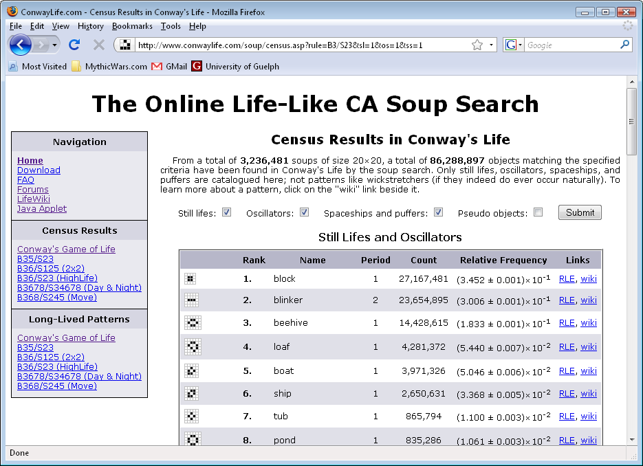
As I mentioned in this post, one way to learn about the general behaviour of Conway’s Game of Life (or any other Life-like cellular automaton) is to generate random patterns and see what stable patterns they typically evolve into (if any). If you’ve played around with Conway’s Game of Life, then you more than likely are very familiar with blocks, blinkers, beehives, loaves, and maybe even pulsars, simply as a result of drawing random gibberish on the grid and letting it evolve. This is exactly the idea behind the Online Life-Like CA Soup Search, just on a larger scale — what if we had lots of people’s computers drawing random gibberish on Life grids, letting them evolve, and storing the resulting patterns in a communal database?

This method of collecting patterns in Life is known as a census, and to my knowledge it has been carried out on a relatively large scale twice in the past; once by Achim Flammenkamp (results here), and once by Andrej Okrasinski (results linked in the first paragraph here). As we would expect, the block is by far the most common still life, and the blinker is by far the most common oscillator. If we scroll down a bit, we see that the pulsar is the fourth most common oscillator (which is reasonably surprising, given its size). Scrolling much past that, we get into the interesting stuff — objects that no reasonable person has ever seen from drawing random stuff and seeing what it evolves into, simply because they occur so infrequently.

So why bother doing another census if two rather large-scale censuses (censi?) have already been carried out? My reasons are threefold:

1. There has never (to my knowledge) been a census of any other Life-like cellular automata conducted. The Online Life-Like CA Soup Search is completely general in that it can conduct a census of any Life-like rule (assuming that rule is stable, of course). Censuses have already been started for five other rules, including 2×2, Day & Night, HighLife, and Move. Because some of these other rules have been studied relatively little, this is an easy way of discovering new yet fundamental patterns in them. For example, it didn’t take long for the soup search script to uncover a c/8 line puffer in the 2×2 (B36/S125) rule; the very first known pattern that exhibits infinite growth in 2×2!
   

   Line puffer in 2×2

2. Previous soup searches were limited in that they only looked for very specific types of objects — usually still lifes and oscillators (though Achim Flammenkamp did a search for spaceships and puffers that can be viewed here). The Online Life-Like CA Soup Search searches for still lifes, oscillators, spaceships and puffers all at once, and even gets pseudo objects (such as the bi-block) as well.
3. Multiple users can run the script and contribute to the results simultaneously. Rather than just having one person run a script that they themself wrote, the Online Life-Like CA Soup Search works by having users download a script and that script uploads results to the central database. This obviously provides a huge speed-up, and allows the census to continuously improve and expand.

So what are you waiting for? Visit the Online Life-Like CA Soup Search, download the script, and put your computer’s CPU cycles to good use!

Census results in Conway’s Game of Life